Runge-Kutta
(2014-12-23)
Differential equations are nasty to deal with. Ideally, an explicit solution can be found, but those may be hard to find, if they exist at all. Numerical solutions, though they produce less mathematical insight, can be applied more generally.
In its most general form, $\frac{d\vec x}{dt} = f(\vec x,t)$. The derivative is given as $\frac{d\vec x}{dt} = \lim_{h \to 0} \frac{\vec x(t+h) - \vec x(t)}{h}$. If we were to pick some small value of $h$, we immediately can find Euler’s method.
$\vec x(t+h) = \vec x(t) + h f(\vec x,t)$
In simplest terms, one applies this by taking the current state, evaluating the derivative, and adding this to the initial value.
Euler’s method is great as a first implementation. However, it is not perfect. The error grows according to $\mathcal{O}(h^2)$. These errors occur whenever the function is not strictly linear.
For example, let us consider $f(x,t) = 2t$, with $x(0) = 0$. This has an explicit solution of $x = t^2$, which we can use as a comparison.
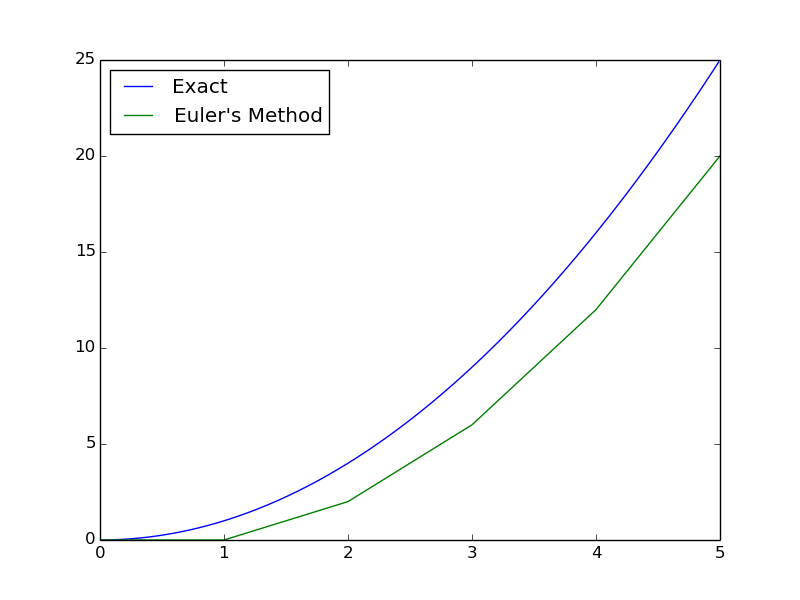
We end up with a very large error, very quickly.
Runge-Kutta is an improved method.[^1] [^1]: Technically, Runge-Kutta is an entire family of methods. The most common of this family, 4th-order Runge-Kutta, is what I will show here. The error is now $\mathcal{O}(h^5)$, rather than the $\mathcal{O}(h^2)$ of Euler’s Method. Remember that $h$ is small, and so a higher exponent means a smaller error. In pseudo-code, Runge-Kutta is implemented as follows.
k1 = h * f(x, t)
k2 = h * f(x + k1/2, t + h/2)
k3 = h * f(x + k2/2, t + h/2)
k4 = h * f(x + k3, t + h)
x(t+h) = x(t) + (k1 + 2*k2 + 2*k3 + k4)/6
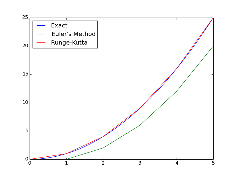
This now requires four function evaluations per step, as opposed to one evaluation per step for Euler’s Method. Runge-Kutta is still more effective, because it can afford to have a larger $h$. The effectiveness of Runge-Kutta is shown below.
Heck, let’s look at a harder case. Let’s have a system of differential equations
$
\frac{dx_1}{dt} = -x_2 \
\frac{dx_2}{dt} = x_1 \
x_1(0) = 1 \
x_2(0) = 0
$
This has an explicit solution of $x_1 = \cos(t)$ and $x_2 = \sin(t)$. Let’s make the same comparison with Euler’s method and Runge-Kutta.
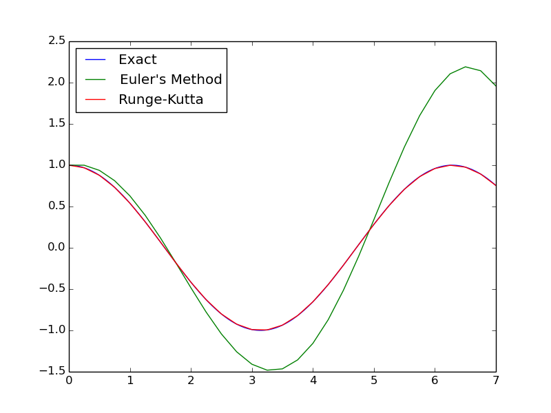
When using Euler’s method, it initially follows the exact solution, but quickly diverges. Runge-Kutta, on the other hand, remains close to the true solution.
Next up, implementation of Runge-Kutta in C++.